Logistic regression
Lecture 10
Duke University
STA 101 - Fall 2023
Warm up
Check-in
- Daily check-ins for getting you thinking at the beginning of the class and reviewing recent/important concepts
- Go to Canvas and open today’s “quiz” titled
2023-10-09 Check-in - Access code:
slopes(released in class) - “Graded” for completion
Project
Project workday on Friday in lab – use this time for finalizing and polishing, not getting started
Projects due Friday at 5 pm
Peer evaluations due Friday at 6 pm:
You’ll receive an email about them later today from TEAMMATES
You must turn in a peer evaluation to get the points your teammates awarded you
Only one person should submit the project on Gradescope and select all team members’ names. See https://sta101-f23.github.io/project/project-1.html#submission for more information.
Any questions about projects?
Logistic regression
So far in regression
Outcome: Numerical, Predictor: One numerical or one categorical with only two levels \(\rightarrow\) Simple linear regression
Outcome: Numerical, Predictors: Any number of numerical or categorical variables with any number of levels \(\rightarrow\) Multiple linear regression
Outcome: Categorical with only two levels, Predictors: Any number of numerical or categorical variables with any number of levels \(\rightarrow\) Logistic regression
Outcome: Categorical with any number of levels, Predictors: Any number of numerical or categorical variables with any number of levels \(\rightarrow\) Generalized linear models – Not covered in STA 101
Data + packages
4601 emails collected at Hewlett-Packard labs and contains 58 variables
Outcome:
typetype = 1is spamtype = 0is non-spam
Predictors of interest:
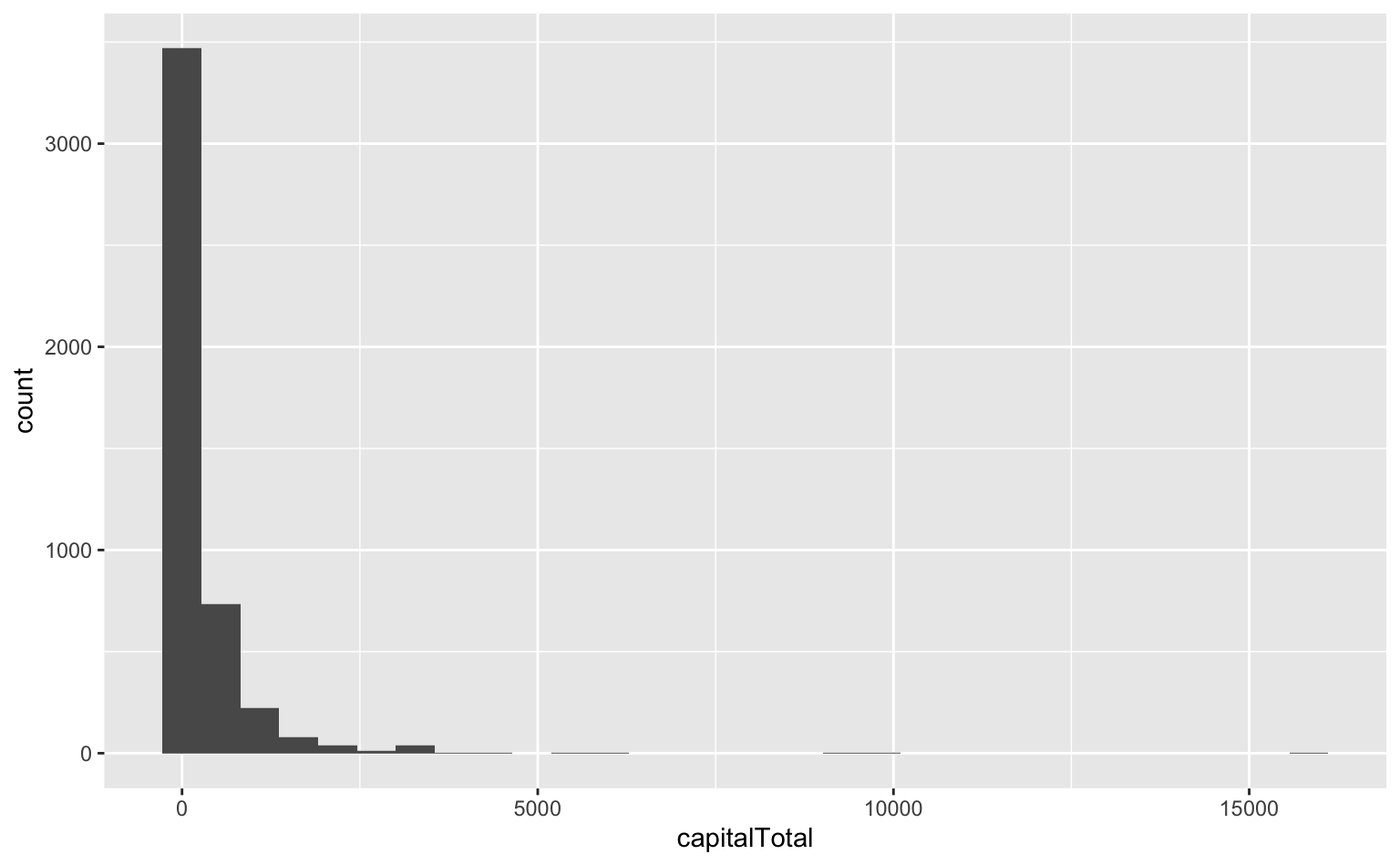
capitalTotal: Number of capital letters in emailPercentages are calculated as (100 * number of times the WORD appears in the e-mail) / total number of words in email
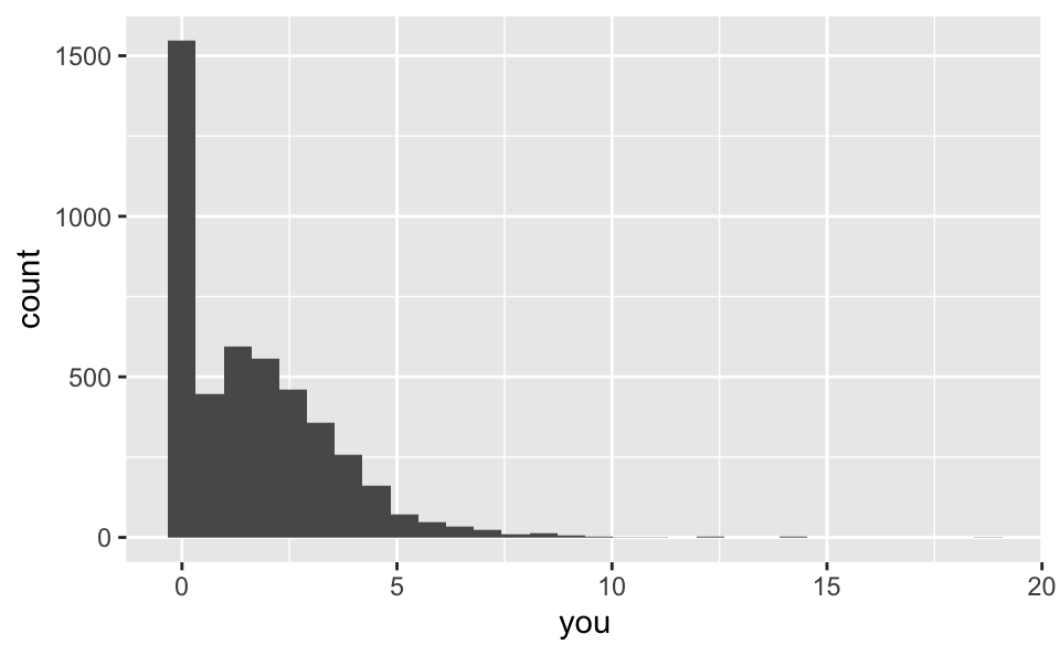
george: Percentage of “george”s in email (these were George’s emails)you: Percentage of “you”s in email
Glimpse at data
What type of data is type? What type should it be in order to use logistic regression?
EDA: How much spam?
EDA: AM I SCREAMING? capitalTotal
EDA: george, is that you?
ggplot(hp_spam, aes(x = george)) +
  geom_histogram()
ggplot(hp_spam, aes(x = you)) +
  geom_histogram()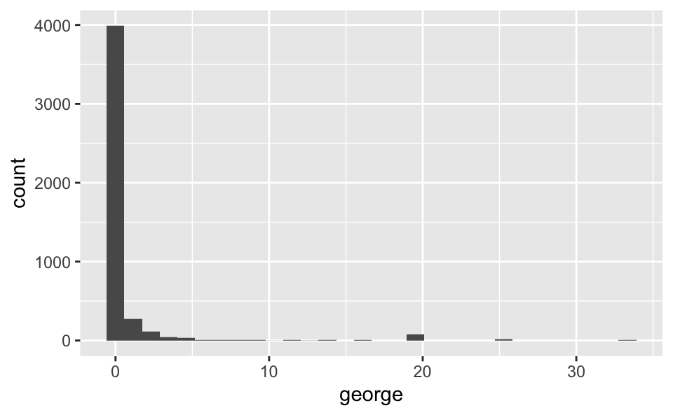
Logistic regression
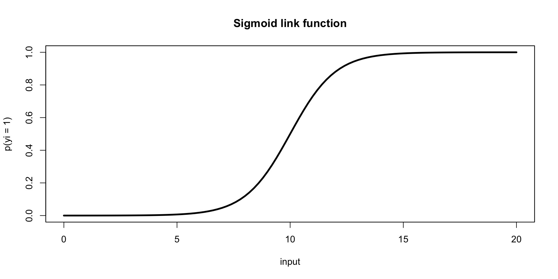
Logistic regression takes in a number of predictors and outputs the probability of a “success” (an outcome of 1) in a binary outcome variable.
The probability is related to the predictors via a sigmoid link function, \[ p(y_i = 1) = \frac{1}{1+\text{exp}({- \sum \beta_i x_i })}, \]whose output is in \((0,1)\) (a probability).
In this modeling scheme, one typically finds \(\hat{\beta}\) by maximizing the likelihood function, another objective function, different than our previous “least squares” objective.
Logistic regression, visualized
Using data to estimate \(\beta_i\)
To proceed with building our email classifier, we will, as usual, use our data (outcome \(y_i\) and predictor \(x_i\) pairs), to estimate \(\beta\) (find \(\hat{\beta}\)) and obtain the model: \[ p(y_i = 1) = \frac{1}{1+\text{exp}({- \sum \hat{\beta}_i x_i})}, \]
Application exercise
Go to Posit Cloud and continue the project titled ae-09-Spam.
ICYMI
Today’s daily check-in access code: slopes (released in class)
