Confidence intervals with bootstrapping
Lecture 13
Duke University
STA 101 - Fall 2023
Warm up
Announcements
Guest lecture on Wednesday with Dr. Yue Jiang – make sure to do the reading before class!
Shopping carts for Spring 2024 open today. If interested in more StatSci courses, I shared info on advising sessions on #random on course Slack.
Packages
From last time…
Case study 1: Donors
Application exercise
Go to Posit Cloud and continue the project titled ae-10-Donor Yawner.
Case study 2: Yawners
Is yawning contagious?
Do you think yawning is contagious?


Is yawning contagious?
An experiment conducted by the MythBusters tested if a person can be subconsciously influenced into yawning if another person near them yawns.
If you’re interested, you can watch the full episode at https://www.dailymotion.com/video/x7ydkt2.
Study description
In this study 50 people were randomly assigned to two groups: 34 to a group where a person near them yawned (treatment) and 16 to a control group where they didn’t see someone yawn (control).
The data are in the openintro package: yawn
Proportion of yawners
# A tibble: 4 × 4
# Groups:   group [2]
  group result       n p_hat
  <fct> <fct>    <int> <dbl>
1 ctrl  not yawn    12 0.75
2 ctrl  yawn         4 0.25
3 trmt  not yawn    24 0.706
4 trmt yawn 10 0.294- Proportion of yawners in the treatment group: \(\frac{10}{34} = 0.2941\)
- Proportion of yawners in the control group: \(\frac{4}{16} = 0.25\)
- Difference: \(0.2941 - 0.25 = 0.0441\)
- Our results match the ones calculated on the MythBusters episode.
Independence?
Based on the proportions we calculated, do you think yawning is really contagious, i.e. are seeing someone yawn and yawning dependent?
# A tibble: 4 × 4
# Groups:   group [2]
  group result       n p_hat
  <fct> <fct>    <int> <dbl>
1 ctrl  not yawn    12 0.75
2 ctrl  yawn         4 0.25
3 trmt  not yawn    24 0.706
4 trmt  yawn        10 0.294
Dependence, or another possible explanation?
- The observed differences might suggest that yawning is contagious, i.e. seeing someone yawn and yawning are dependent.
- But the differences are small enough that we might wonder if they might simple be due to chance.
- Perhaps if we were to repeat the experiment, we would see slightly different results.
- So we will do just that - well, somewhat - and see what happens.
- Instead of actually conducting the experiment many times, we will simulate our results.
Two competing claims
Null hypothesis:
“There is nothing going on.” Yawning and seeing someone yawn are independent, yawning is not contagious, observed difference in proportions is simply due to chance.
Alternative hypothesis:
“There is something going on.” Yawning and seeing someone yawn are dependent, yawning is contagious, observed difference in proportions is not due to chance.
Simulation by hand - setup
A regular deck of cards is comprised of 52 cards: 4 aces, 4 of numbers 2-10, 4 jacks, 4 queens, and 4 kings.
Take out two aces from the deck of cards and set them aside.
The remaining 50 playing cards to represent each participant in the study:
- 14 face cards (including the 2 aces) represent the people who yawn.
- 36 non-face cards represent the people who don’t yawn.
Simulation by hand - running
Shuffle the 50 cards at least 7 times1 to ensure that the cards counted out are from a random process.
Count out the top 16 cards and set them aside. These cards represent the people in the control group.
Out of the remaining 34 cards (treatment group) count the number of face cards (the number of people who yawned in the treatment group).
Calculate the difference in proportions of yawners (treatment - control), and record that value.
Repeat steps 1-4 many times (100, 1000, 15000, …) to build the null distribution of differences in proportions of yawners.
Simulation by computation
Go to Posit Cloud and continue the project titled ae-10-Donor Yawner.
Recap
Types of alternative hypotheses
- One-sided (one-tailed) alternatives: The parameter is hypothesized to be less than or greater than the null value, < or >
- Two-sided (two-tailed) alternatives: The parameter is hypothesized to be not equal to the null value, \(\ne\)
- Calculated as two times the tail area beyond the observed sample statistic
- More objective, and hence more widely preferred
Average systolic blood pressure of people with Stage 1 Hypertension is 150 mm Hg. Suppose we want to use a hypothesis test to evaluate whether a new blood pressure medication has an effect on the average blood pressure of heart patients. What are the hypotheses?
Discernability level
We often use 5% as the cutoff for whether the p-value is low enough that the data are unlikely to have come from the null model. This cutoff value is called the discernability level, \(\alpha\).
If p-value < \(\alpha\), reject \(H_0\) in favor of \(H_A\): The data provide convincing evidence for the alternative hypothesis.
If p-value > \(\alpha\), fail to reject \(H_0\) in favor of \(H_A\): The data do not provide convincing evidence for the alternative hypothesis.
Statistically discernable
If you’ve taken a statistics course before, or read papers that use hypothesis testing for making a conclusion, you might have encountered the term “statistically significant” or “significance level”.
We will use the term “statistically discernable” or discernability level”, because “significant” has a different meaning in everyday language and this often causes misconceptions of what “statistically significant” means. It doesn’t necessarily mean a notable or important event has happened, it just means the data are unlikely to have come from the null model.
Setting a seed
Goal: Pin down the random generation so that the same random generation happens each time a document is rendered (by you or by someone else wanting to replicate your results)
When: Set a seed each time right before
generate()ing new resamples. Setting a seed once in a document would also work for re-rendering the document, but considering we often run the code chunk interactively, it’s best to set the seed again in each code chunk that does random generation.
Confidence intervals
Case study 3: Airbnb in Asheville, NC
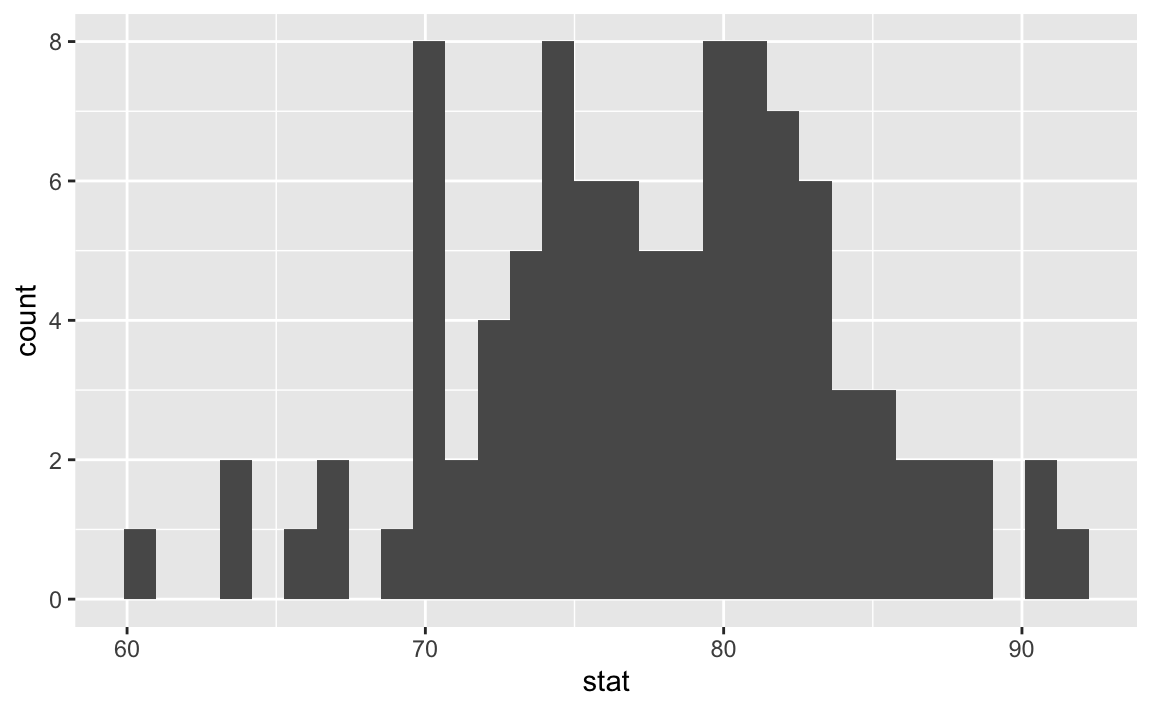
We have data on the price per guest (ppg) for a random sample of 50 Airbnb listings in 2020 for Asheville, NC. We are going to use these data to investigate what we would of expected to pay for an Airbnb in in Asheville, NC in June 2020.
Terminology
Population parameter - What we are interested in. Statistical measure that describes an entire population.
Sample statistic (point estimate) - describes a sample. A piece of information you get from a fraction of the population.
Catching a fish
Suppose you’re fishing in a murky lake. Are you more likely to catch a fish using a spear or a net?
- Spear \(\rightarrow\) point estimate
- Net \(\rightarrow\) interval estimate
Constructing confidence intervals
Quantifying the variability of the sample statistics to help calculate a range of plausible values for the population parameter of interest:
Via simulation \(\rightarrow\) using bootstrapping – using a statistical procedure that re samples a single data set to create many simulated samples.
Via mathematical formulas \(\rightarrow\) using the Central Limit Theorem
Bootstrapping, what?
The term bootstrapping comes from the phrase “pulling oneself up by one’s bootstraps”, which is a metaphor for accomplishing an impossible task without any outside help.
Impossible task: estimating a population parameter using data from only the given sample.
Note
Note: This notion of saying something about a population parameter using only information from an observed sample is the crux of statistical inference, it is not limited to bootstrapping.
Bootstrapping, how?
- Resample with replacement from our data n times, where n is the sample size
- Calculate the sample statistic of interest of the new, resampled (bootstrapped) sample and record the value
- Do this entire process many many times to build the bootstrap distribution
Bootstrapping Airbnb rentals
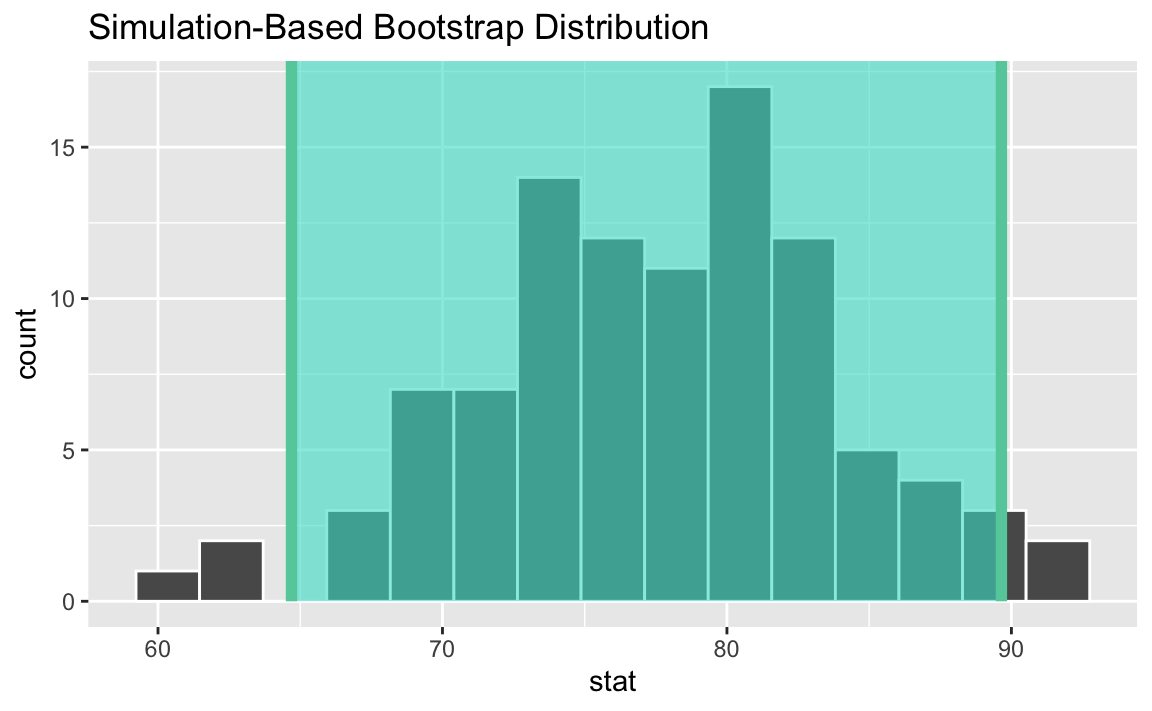
The bootstrap distribution
Visualzing the bootstrap distribution
What do you expect the center of the bootstrap distribution to be? Why? Check your guess by visualizing the distribution.
Calculating the bootstrap distribution
Interpretation
Which of the following is the correct interpretation of the bootstrap interval?
Reply on Canvas in “2023-10-23 Check-in” with access code bootstrap.
There is a 95% probability the true mean price per night for an Airbnb in Asheville is between $64.7 and $89.6.
There is a 95% probability the price per night for an Airbnb in Asheville is between $64.7 and $89.6.
We are 95% confident the true mean price per night for Airbnbs in Asheville is between $64.7 and $89.6.
We are 95% confident the price per night for an Airbnb in Asheville is between $64.7 and $89.6.
Leveraging tidymodels tools further
Calculating the observed sample statistic:
Leveraging tidymodels tools further
Calculating the interval:
Leveraging tidymodels tools further
Visualizing the interval:
![]()