Inference with mathematical models

Lecture 15

Dr. Mine Çetinkaya-Rundel

Duke University
STA 101 - Fall 2023

Warm up

Announcements

  • My office hours by appointment this week.
  • Wednesday lecture on Zoom – can join from wherever, will send Zoom link by email and on Slack.

Packages

library(tidyverse)
library(tidymodels)
library(openintro)

Inference with mathematical models

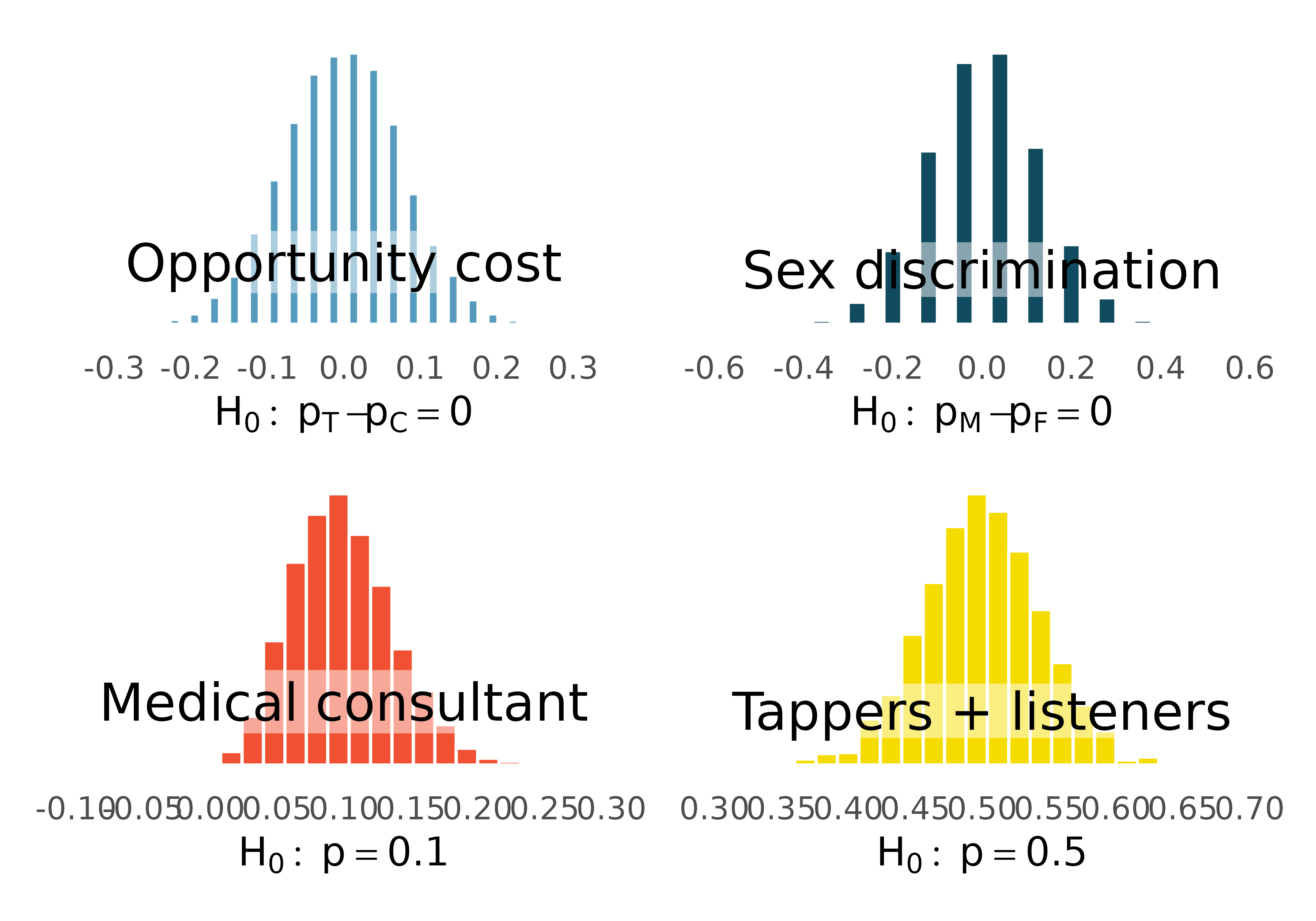
That familiar shape…

Describe the shape of the distributions.

It’s not happenstance!

It’s the Central Limit Theorem, which says that the distribution of the sample statistic is normal, if certain conditions are met.

Two questions:

  1. What do we mean by the distribution of the sample statistic?
  2. What conditions need to be met?

The distribution of the sample statistic

  • You can build the distribution of the sample statistic by repeatedly taking samples of size n (original sample size) from the population and calculating and recording the sample statistic for each of these samples.

  • But, you would never do this in reality!

  • You’d either use simulation (randomization, bootstrapping, stuff we’ve done so far!) or you would leverage mathematical theory to know what to expect if we had taken repeated samples.

The (technical) conditions

  1. Independent observations: Observations in the sample are independent. Independence is guaranteed when we take a random sample from a population. Independence can also be guaranteed if we randomly divide individuals into treatment and control groups.

  2. Large enough sample: The sample size cannot be too small. What qualifies as “small” differs from one context (i.e., from sample statistic to sample statistic).

More to the CLT

  • There is more to the CLT than just the shape of the distribution – normal.

  • The CLT says that the center of the sampling distribution will be at the true population parameter.

  • The CLT also says something about the spread of the sampling distribution, measured by the standard error. For each sample statistic (\(\bar{x}\) – the sample mean, \(\hat{p}\) – the sample proportion, \(\bar{x}_1 - \bar{x}_2\) – the difference in sample means, etc.) the CLT provides a formula for its standard error.

    • You won’t be asked to memorize these formulas.

    • In fact, you’ll rarely use the CLT to calculate the variability of sample statistics, you’ll simulate their distributions directly.

Normal distribution

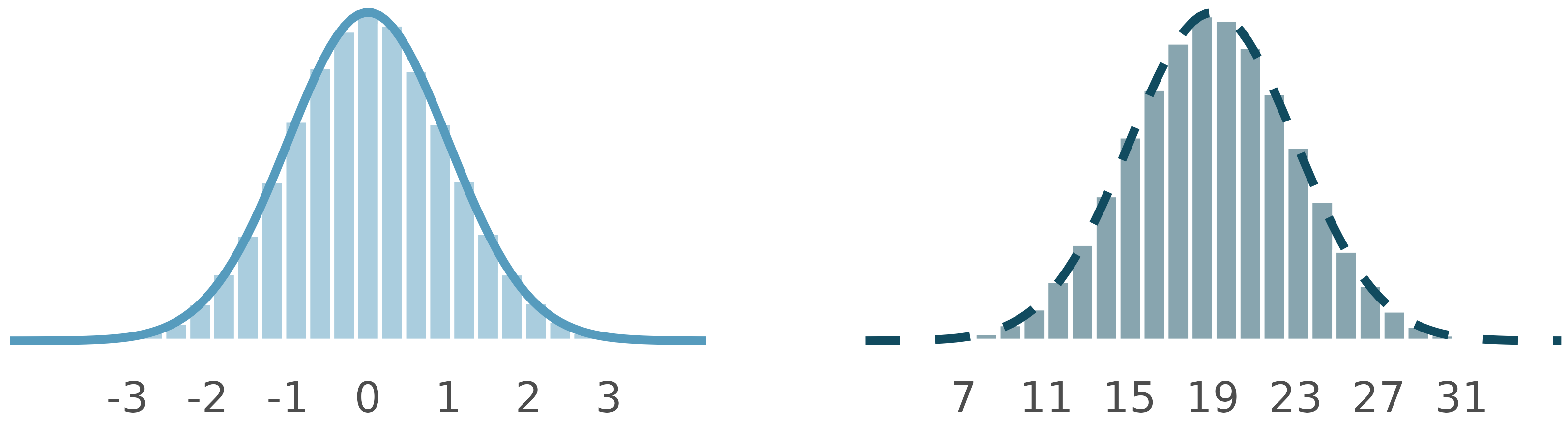
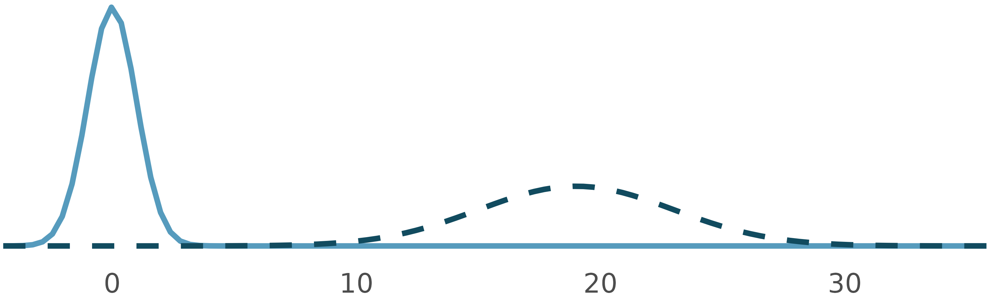
Normal distributions

How are these normal distributions similar? How are they different? Which one is \(N(\mu = 0, \sigma. 1)\) and which \(N(\mu = 19, \sigma = 4)\)?
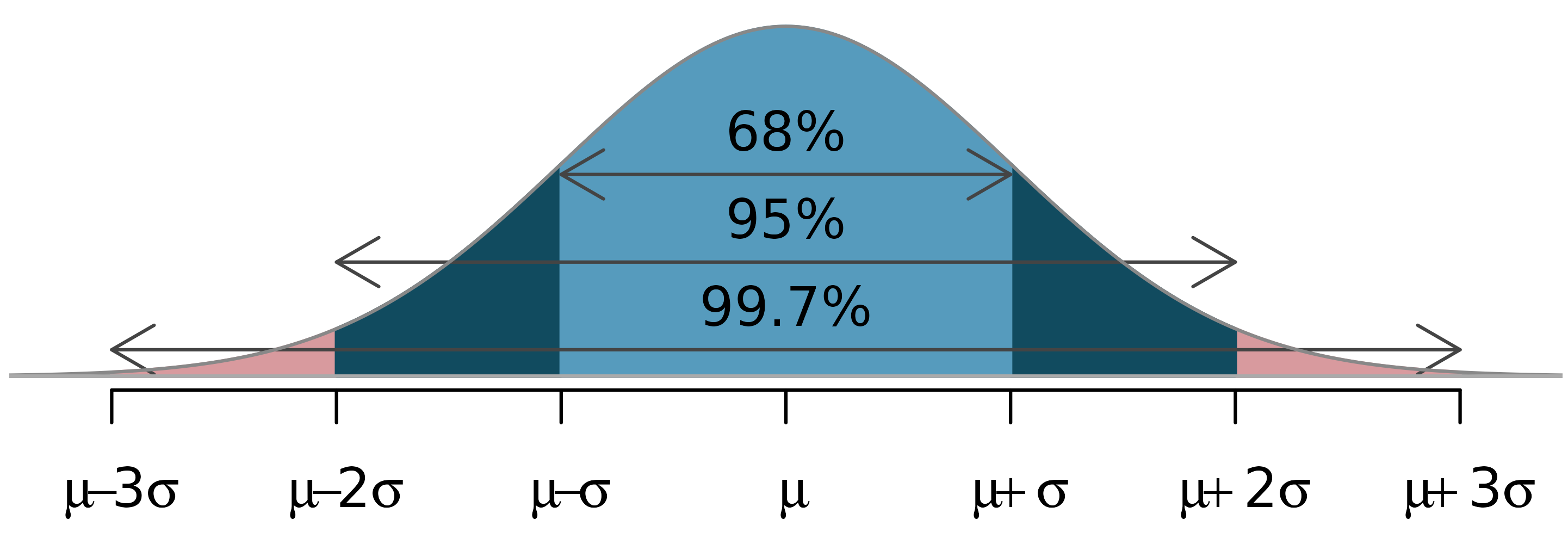
The 68-95-99.7 rule

The normal distribution is not just any unimodal and symmetric distribution, it follows the 68-95-99.7 rule.

Using the normal distribution…

  • To make decisions \(\rightarrow\) hypothesis testing

    • Use properties of the normal distribution to determine the probability of the observed sample statistic (or something more extreme, in the direction of the alternative hypothesis), i.e. the p-value
  • To make estimations \(\rightarrow\) confidence intervals

    • Use properties of the normal distribution to calculate the bounds of the confidence interval, adding and subtracting a margin of error to the observed sample statistic

But before then…

Application exercise

Go to Posit Cloud and continue the project titled ae-11-Bone density.