library(tidyverse)
library(tidymodels)
library(DAAG)Weights of books
Application exercise
Suggested answers
Important
These are suggested answers for the application exercise. They’re not necessarily complete or 100% accurate, they’re roughly what we develop in class while going through the exercises.
Today we’ll explore the question “How do volume and weights books relate?” and “How, if at all, does that change when we take whether the book is hardback or paperback into consideration?”
Goals
Build, fit, and interpret linear models with more than one predictor
Use categorical variables as a predictor in a model
Compute \(R^2\) and use it to select between models
Packages
Data
The data for this application exercise comes from the allbacks dataset in the DAAG package. The dataset has 15 observations and 4 columns. Each observation represents a book. Let’s take a peek at the data:
allbacks volume area weight cover
1 885 382 800 hb
2 1016 468 950 hb
3 1125 387 1050 hb
4 239 371 350 hb
5 701 371 750 hb
6 641 367 600 hb
7 1228 396 1075 hb
8 412 0 250 pb
9 953 0 700 pb
10 929 0 650 pb
11 1492 0 975 pb
12 419 0 350 pb
13 1010 0 950 pb
14 595 0 425 pb
15 1034 0 725 pbNote that volume is measured in cubic centimeters and weight is measured in grams. More information on the dataset can be found in the documentation for allbacks, with ?allbacks.
Single predictor
Exercise 1
Visualize the relationship between volume (on the x-axis) and weight (on the y-axis). Overlay the line of best fit. Describe the relationship between these variables.
ggplot(allbacks, aes(x = volume, y = weight)) +
  geom_point() +
  geom_smooth(method = "lm", se = FALSE) +
  labs(
    x = "Volume (cubic centimeters)",
    y = "Weight (grams)"
  )
`geom_smooth()` using formula = 'y ~ x'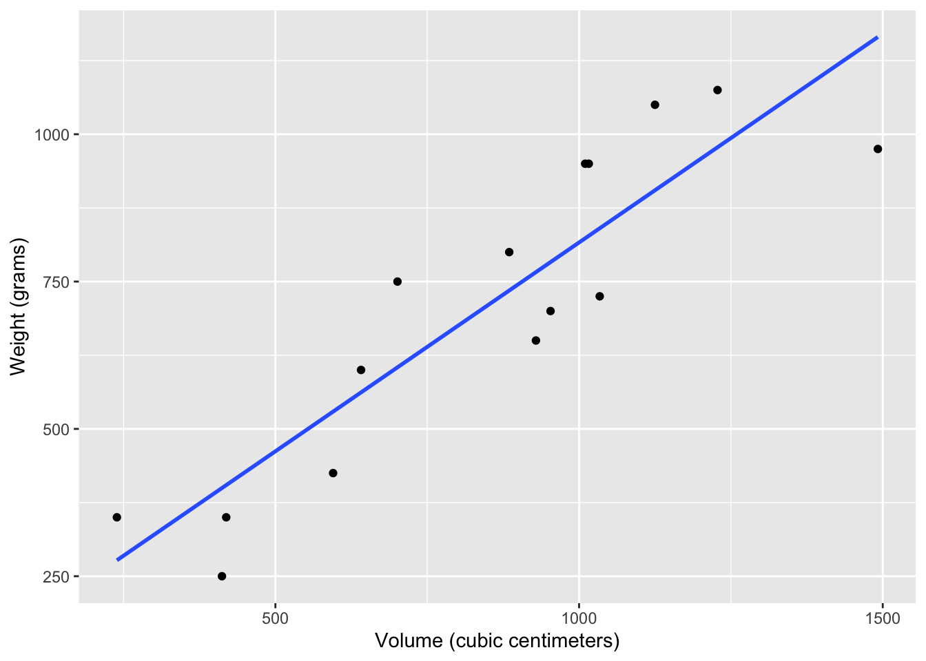
Exercise 2
Fit a model predicting weight from volume for these books and save it as weight_fit. Display a tidy output of the model.
weight_fit <- linear_reg() |>
  fit(weight ~ volume, data = allbacks)

tidy(weight_fit)
# A tibble: 2 × 5
term estimate std.error statistic p.value
<chr> <dbl> <dbl> <dbl> <dbl>
1 (Intercept) 108. 88.4 1.22 0.245
2 volume 0.709 0.0975 7.27 0.00000626Exercise 3
Interpret the slope and the intercept in context of the data.
Intercept: Books with 0 volume are expected, on average, to weigh approximately 107.68 grams. This doesn’t make sense in the context of the data, and the intercept is only there to adjust the height of the line on the y-axis.
Slope: For each additional cubic centimeter the book’s volume is larger, we expect the weight to be higher, on average, by 0.71 grams.
Exercise 4
Calculate the \(R^2\) of this model and interpret it in context of the data.
glance(weight_fit)# A tibble: 1 × 12
r.squared adj.r.squared sigma statistic p.value df logLik AIC BIC
<dbl> <dbl> <dbl> <dbl> <dbl> <dbl> <dbl> <dbl> <dbl>
1 0.803 0.787 124. 52.9 0.00000626 1 -92.5 191. 193.
# ℹ 3 more variables: deviance <dbl>, df.residual <int>, nobs <int>Volume explains approximately 80% of the variability in book weights.
Multiple predictors
Exercise 5
Visualize the relationship between volume (on the x-axis) and weight (on the y-axis), taking into consideration the cover type of the book. Use different colors and shapes for hardback and paperback books. Also use different colors for lines of best fit for the two types of books. In addition, add the overall line of best fit (from Exercise 1) as a gray dashed line so that you can see the difference between the lines when considering and not considering cover type.
ggplot(allbacks, aes(x = volume, y = weight)) +
  geom_smooth(method = "lm", se = FALSE, color = "gray", linetype = "dashed") +
  geom_point(aes(color = cover, shape = cover)) +
  geom_smooth(aes(color = cover), method = "lm", se = FALSE) +
  labs(
    x = "Volume (cubic centimeters)",
    y = "Weight (grams)",
    shape = "Cover", color = "Cover"
  )
`geom_smooth()` using formula = 'y ~ x'
`geom_smooth()` using formula = 'y ~ x'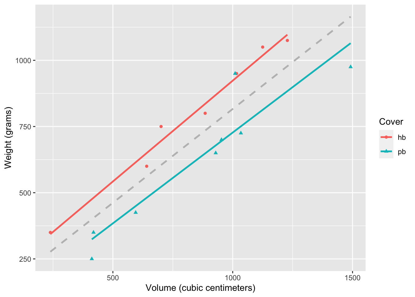
Exercise 6
Fit a model predicting weight from volume for these books and save it as weight_cover_fit. Display a tidy output of the model.
weight_cover_fit <- linear_reg() |>
  fit(weight ~ volume + cover, data = allbacks)

tidy(weight_cover_fit)
# A tibble: 3 × 5
term estimate std.error statistic p.value
<chr> <dbl> <dbl> <dbl> <dbl>
1 (Intercept) 198. 59.2 3.34 0.00584
2 volume 0.718 0.0615 11.7 0.0000000660
3 coverpb -184. 40.5 -4.55 0.000672 Exercise 7
In the model output we have a variable coverpb. Why is only the pb (paperback) level of the cover variable shown? What happened to the hb (hardback) level?
Hardback is the reference level, therefore doesn’t show up in the model output.
Exercise 8
Interpret the slopes and the intercept in context of the data.
Intercept: Books with 0 volume and that are hardback are expected, on average, to weigh approximately 197.96 grams. This doesn’t make sense in the context of the data, and the intercept is only there to adjust the height of the line on the y-axis.
Slope - volume: All else held constant, for each additional cubic centimeter the book’s volume is larger, we expect the weight to be higher, on average, by 0.72 grams.
Slope - cover: All else held constant, paperback books weigh, on average, 184.05 grams lower than harback books.
Exercise 9
First, guess whether the \(R^2\) of this model will be greater than, less than, or the same as the previous model, or whether we can’t tell. Then, calculate the \(R^2\) of this model to confirm your guess, and then interpret it in context of the data.
glance(weight_cover_fit)# A tibble: 1 × 12
r.squared adj.r.squared sigma statistic p.value df logLik AIC BIC
<dbl> <dbl> <dbl> <dbl> <dbl> <dbl> <dbl> <dbl> <dbl>
1 0.927 0.915 78.2 76.7 0.000000145 2 -85.0 178. 181.
# ℹ 3 more variables: deviance <dbl>, df.residual <int>, nobs <int>\(R^2\) of this model will be higher since it has an additional predictor.
Volume and cover type explain approximately 93% of the variability in book weights.
Exercise 10
Which model is preferred for predicting book weights and why?
The second model, since it has a higher adjusted \(R^2\).
Exercise 11
Using the model you chose, predict the weight of a hardcover book that is 1000 cubic centimeters (that is, roughly 25 centimeters in length, 20 centimeters in width, and 2 centimeters in height/thickness).
new_book <- tibble(
  cover = "hb",
  volume = 1000
)

predict(weight_cover_fit, new_data = new_book)
# A tibble: 1 × 1
.pred
<dbl>
1 916.