library(tidyverse)
library(tidymodels)
library(openintro)Donors and yawners
Application exercise
Suggested answers
In this application exercise, we’ll introduce pipelines for conducting hypothesis tests with randomization.
Goals
Conduct a hypothesis test for a proportion
Conduct a hypothesis test for a difference in proportions
Packages and data
We’ll use the tidyverse and tidymodels packages as usual and the openintro package for the datasets.
Case study 1: Donors
The first dataset we’ll use is organ_donors, which is in your data folder:
organ_donor <- read_csv("data/organ-donor.csv")Rows: 62 Columns: 1
── Column specification ────────────────────────────────────────────────────────
Delimiter: ","
chr (1): outcome
ℹ Use `spec()` to retrieve the full column specification for this data.
ℹ Specify the column types or set `show_col_types = FALSE` to quiet this message.The hypotheses we are testing are:
\(H_0: p = 0.10\)
\(H_A: p \ne 0.10\)
where \(p\) is the true complication rate for this consultant.
Exercise 1
Construct the null distribution with 100 resamples. Name it null_dist_donor. How many rows does null_dist_donor have? How many columns? What does each row and each column represent?
set.seed(25)

null_dist_donor <- organ_donor |>
  specify(response = outcome, success = "complication") |>
  hypothesize(null = "point", p = 0.10) |>
  generate(reps = 100, type = "draw") |>
  calculate(stat = "prop")

null_dist_donor
Response: outcome (factor)
Null Hypothesis: point
# A tibble: 100 × 2
replicate stat
<fct> <dbl>
1 1 0.0645
2 2 0.0484
3 3 0.113
4 4 0.0806
5 5 0.145
6 6 0.145
7 7 0.113
8 8 0.0806
9 9 0.113
10 10 0.145
# ℹ 90 more rows
null_dist_donorhas 100 rows and 2 columns. Each row is a replicate, andreplicatecolumn indicates the replicate number andstatis the simulated proportion, \(\hat{p}\).
Exercise 2
Where do you expect the center of the null distribution to be? Visualize it to confirm.
# option 1
ggplot(null_dist_donor, aes(x = stat)) +
  geom_histogram(bins = 15, color = "white")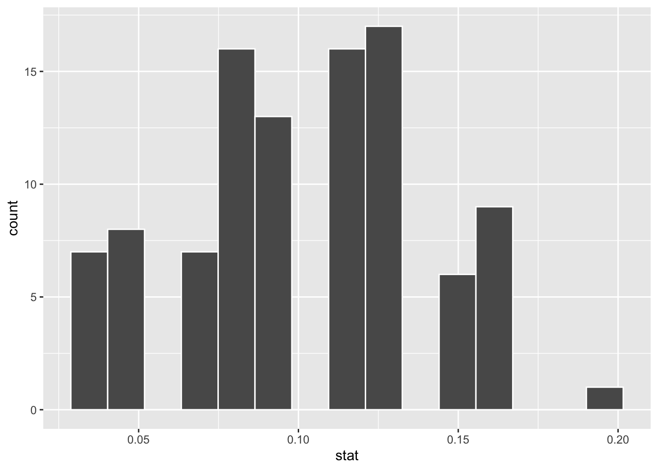
# option 2
visualize(null_dist_donor)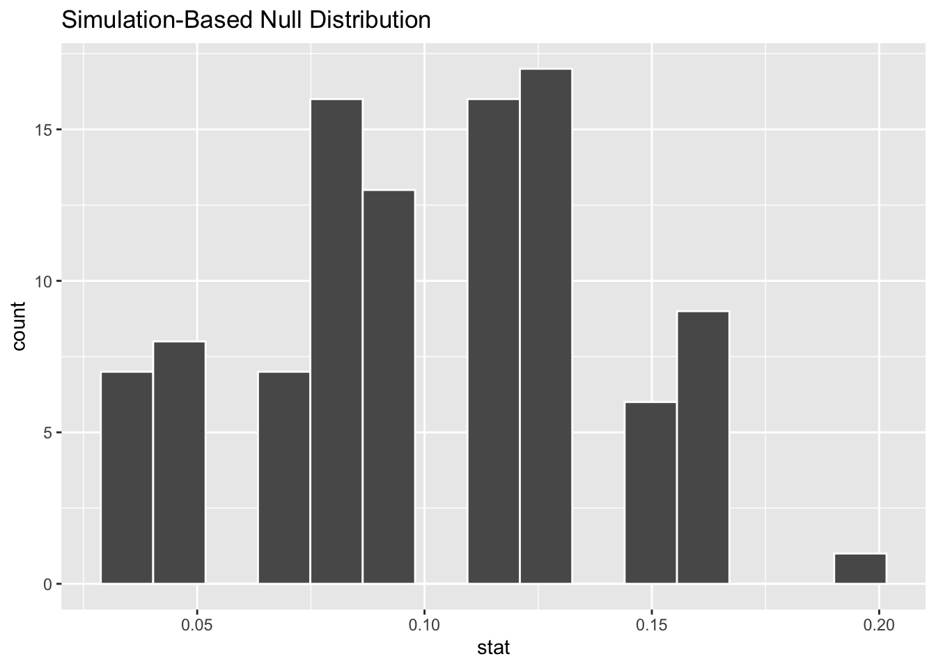
Exercise 2
Calculate the observed complication rate of this consultant. Name it obs_stat_donor.
obs_stat_donor <- organ_donor |>
  specify(response = outcome, success = "complication") |>
  calculate(stat = "prop")

obs_stat_donor
Response: outcome (factor)
# A tibble: 1 × 1
stat
<dbl>
1 0.0484Exercise 3
Overlay the observed statistic on the null distribution and comment on whether an observed outcome as extreme as the observed statistic, or lower, is a likely or unlikely outcome, if in fact the null hypothesis is true.
# option 1
ggplot(null_dist_donor, aes(x = stat)) +
  geom_histogram(bins = 15, color = "white") +
  geom_vline(xintercept = obs_stat_donor |> pull(stat), color = "red", linewidth = 2)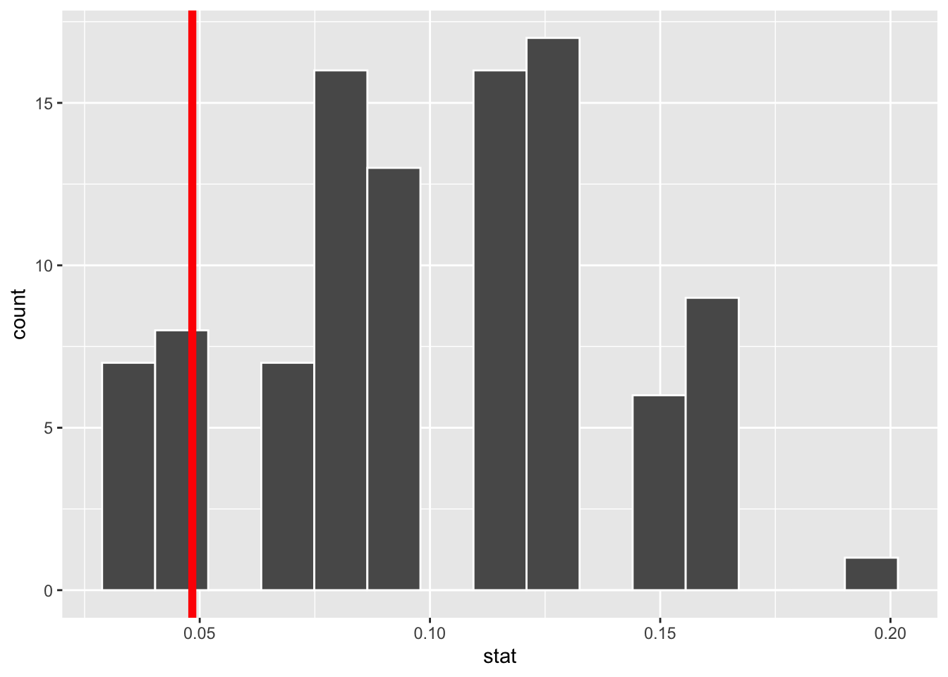
# option 2
visualize(null_dist_donor) +
  shade_p_value(obs_stat = obs_stat_donor, direction = "two-sided")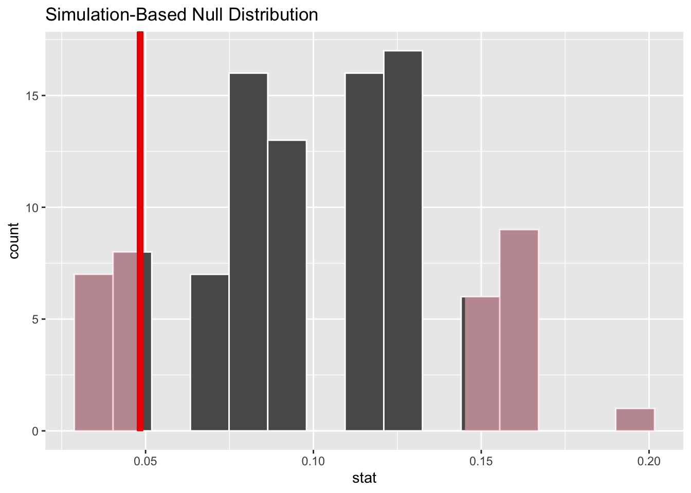
Exercise 4
Calculate the p-value and comment on whether it provides convincing evidence that this consultant incurs a lower complication rate than 10% (overall US complication rate).
Since the p-value is greater than the discernability level, we fail to reject the null hypothesis. These data do not provide convincing evidence that this consultant incurs a lower complication rate than 10% (overall US complication rate).
# option 1
null_dist_donor |>
  filter(stat <= obs_stat_donor |> pull(stat)) |>
  nrow()*2 / 100
[1] 0.3# option 2
null_dist_donor |>
get_p_value(obs_stat = obs_stat_donor, direction = "two-sided")# A tibble: 1 × 1
p_value
<dbl>
1 0.3Exercise 5
Let’s get real! Redo the test with 15,000 simulations. Note: This can take some time to run.
set.seed(25)

null_dist_donor <- organ_donor |>
  specify(response = outcome, success = "complication") |>
  hypothesize(null = "point", p = 0.10) |>
  generate(reps = 15000, type = "draw") |>
  calculate(stat = "prop")

null_dist_donor |>
  visualize() +
  shade_p_value(obs_stat = obs_stat_donor, direction = "two-sided")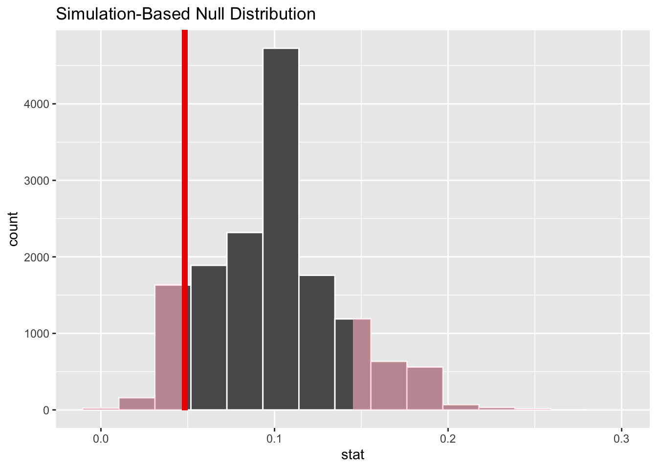
null_dist_donor |>
  get_p_value(obs_stat = obs_stat_donor, direction = "two-sided")
# A tibble: 1 × 1
p_value
<dbl>
1 0.241Case study 2: Yawners
Exercise 6
Using the yawn dataset in the openintro package, conduct a hypothesis test for evaluating whether yawning is contagious. First, set the hypotheses. Then, conduct a randomization test using 1000 simulations. Visualize and calculate the p-value and use it to make a conclusion about the statistical discernability of the difference in proportions of yawners in the two groups. Then, comment on whether you “buy” this conclusion.
Null hypothesis: Yawning is not contagious; \(p_{trmt} = p_{ctrl}\) Alternative hypothesis: Yawning is contagious; \(p_{trmt} > p_{ctrl}\) With a p-value 0.522, which is much larger than the discernability level of 0.05, we fail to reject the null hypothesis. These data do not provide convincing evidence that yawning is contagious. Frankly, I don’t buy this statement. I think yawning is contagious. This could be an example of a hypothesis testing error where we fail to reject the null hypothesis when we should have, i.e., a Type II error.
set.seed(25)

null_dist_yawner <- yawn |>
  specify(response = result, explanatory = group, success = "yawn") |>
  hypothesize(null = "independence") |>
  generate(reps = 1000, type = "permute") |>
  calculate(stat = "diff in props", order = c("trmt", "ctrl"))

obs_stat_yawner <- yawn |>
  specify(response = result, explanatory = group, success = "yawn") |>
  calculate(stat = "diff in props", order = c("trmt", "ctrl"))

null_dist_yawner |>
  visualize() +
  shade_p_value(obs_stat = obs_stat_yawner, direction = "greater")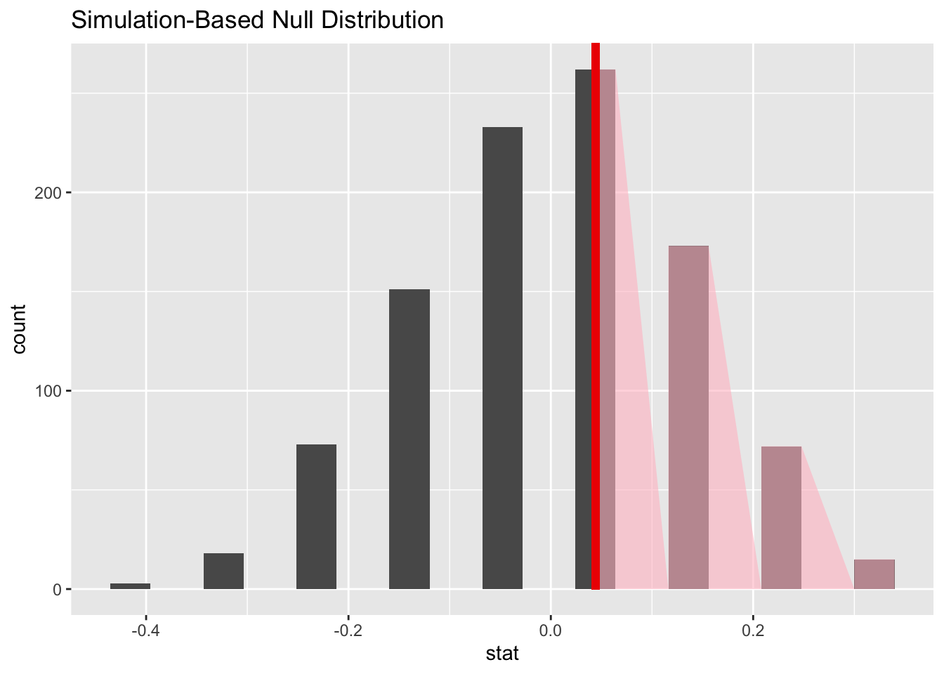
null_dist_yawner |>
  get_p_value(obs_stat = obs_stat_yawner, direction = "greater")
# A tibble: 1 × 1
p_value
<dbl>
1 0.522