library(tidyverse)
library(openintro)
Bone density
Application exercise
Suggested answers
In this application exercise, we’ll introduce and work with the normal distribution.
Goals
Calculate probabilities under the normal curve
Understand Z scores
Build intuition for hypothesis testing and confidence interval building with the normal distribution
Packages and data
We’ll use the tidyverse and openintro packages.
Bone density - population
Suppose the bone density for 65-year-old women is normally distributed with mean 809 \(mg/cm^3\) and standard deviation of 140 \(mg/cm^3\).
Let \(x\) be the bone density of 65-year-old women. We can write this distribution of \(x\) in mathematical notation as
\[ x \sim N(\mu = 809, \sigma = 140) \]
Let’s set the parameters of this distribution as objects you can use later.
bone_density_mean <- 809
bone_density_sd <- 140
Exercise 1
Visualize the distribution of bone density of 65-year-old women.
# option 1: ggplot2
ggplot(
  data = tibble(x = c(bone_density_mean - bone_density_sd*3, bone_density_mean + bone_density_sd*3)),
  aes(x = x)) +
  stat_function(
    fun = dnorm,
    args = list(mean = bone_density_mean, sd = bone_density_sd)
  )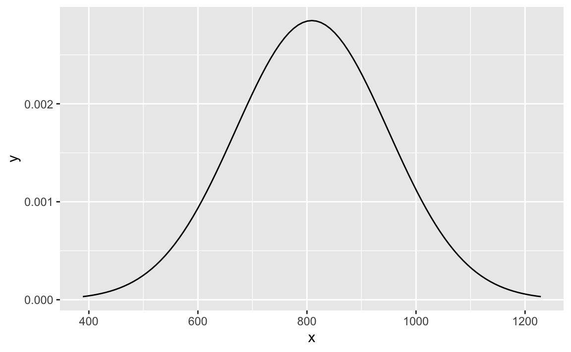
# option 2: openintro -- shortcut
normTail(m = bone_density_mean, s = bone_density_sd)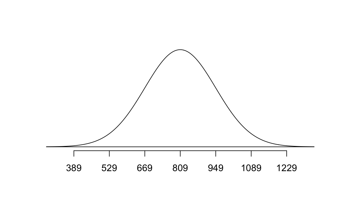
Exercise 2
Before typing any code, based on what you know about the normal distribution, what do you expect the median bone density to be?
809 \(mg/cm^3\), since mean and median are roughly equal for symmetric distributions.
Exercise 3
What bone densities correspond to Q1 (25th percentile), Q2 (50th percentile), and Q3 (the 75th percentile) of this distribution? Use the qnorm() function to calculate these values.
qnorm(p = 0.25, mean = bone_density_mean, sd = bone_density_sd)[1] 714.5714qnorm(p = 0.50, mean = bone_density_mean, sd = bone_density_sd)[1] 809qnorm(p = 0.75, mean = bone_density_mean, sd = bone_density_sd)[1] 903.4286Exercise 4
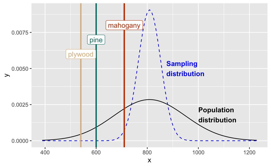
The densities of three woods are below:
Plywood: 540 \(mg/cm^3\)
Pine: 600 \(mg/cm^3\)
Mahogany: 710 \(mg/cm^3\)
Let’s set these as variables we can use later:
plywood <- 540
pine <- 600
mahogany <- 710
What is the probability that a randomly selected 65-year-old woman has bones less dense than Pine?
normTail(m = bone_density_mean, s = bone_density_sd, L = pine)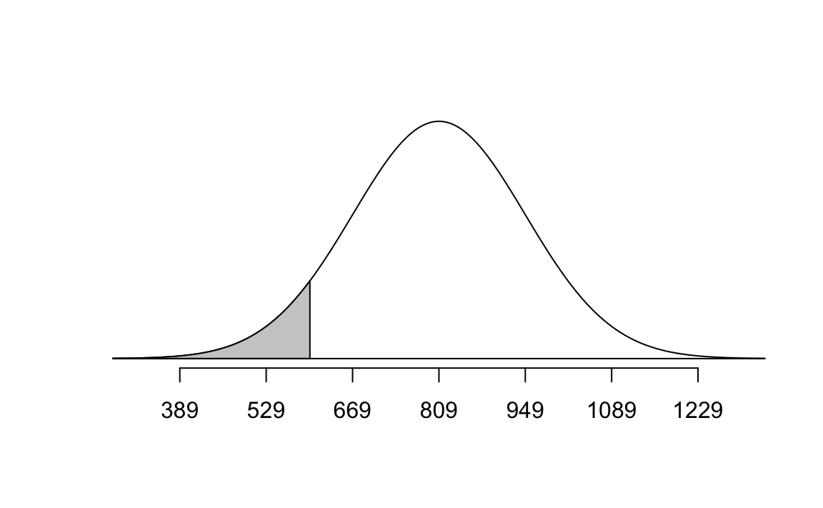
pnorm(q = pine, mean = bone_density_mean, sd = bone_density_sd)[1] 0.06773729Exercise 5
Would you be surprised if a randomly selected 65-year-old woman had bone density less than Mahogany? What if she had bone density less than Plywood? Use the respective probabilities to support your response.
No for Mahogany, yes for Plywood.
# Mahogany
normTail(m = bone_density_mean, s = bone_density_sd, L = mahogany)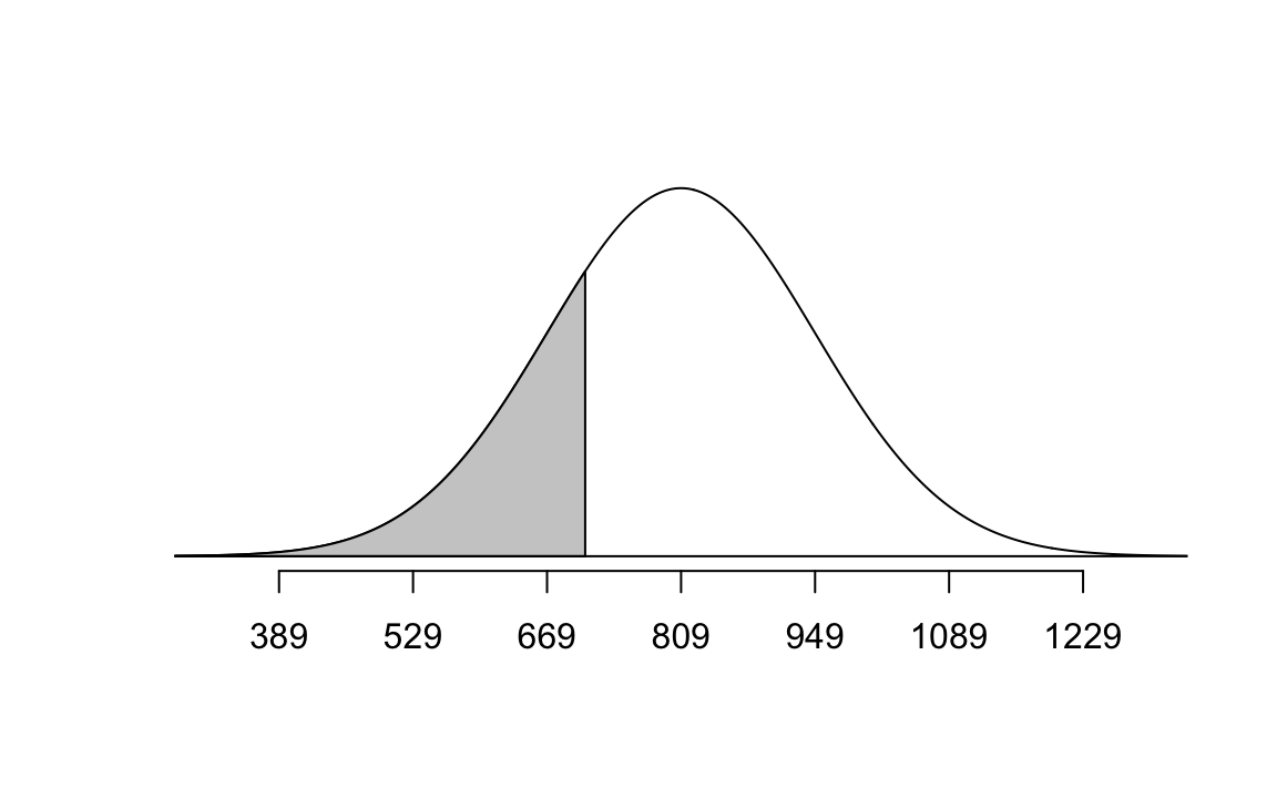
pnorm(q = mahogany, mean = bone_density_mean, sd = bone_density_sd)[1] 0.2397389# Plywood
normTail(m = bone_density_mean, s = bone_density_sd, L = plywood)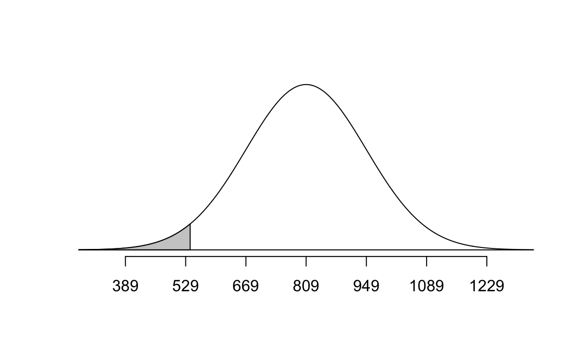
pnorm(q = plywood, mean = bone_density_mean, sd = bone_density_sd)[1] 0.02733885Bone density - sampling
Suppose you want to analyze the mean bone density for a group of 10 randomly selected 65-year-old women.
Exercise 6
Are the conditions for the Central Limit Theorem met?
Independence: Yes, random sampling.
Sample size/distribution: Yes, sample size is small, but the population distribution is normal, so the sampling distribution will be a well.
Exercise 7
What is the shape, center, and spread of the distribution of the mean bone density for a group of 10 randomly selected 65-year-old women?
\[ \bar{x} \sim N(mu = 809, SE = 140 / \sqrt{10} \approx 44) \]
Exercise 8
What is the probability that the mean bone density for the group of 10 randomly-selected 65-year-old women is less dense than Pine?
bone_density_se <- 44

normTail(m = bone_density_mean, s = bone_density_se, L = pine)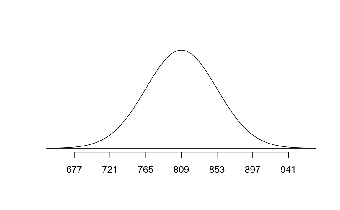
pnorm(q = pine, mean = bone_density_mean, sd = bone_density_se)[1] 1.017083e-06Exercise 9
Would you be surprised if a group of 10 randomly-selected 65-year old women had a mean bone density less than Mahogany? What the group had a mean bone density less than Plywood? Use the respective probabilities to support your response.
normTail(m = bone_density_mean, s = bone_density_se, L = mahogany)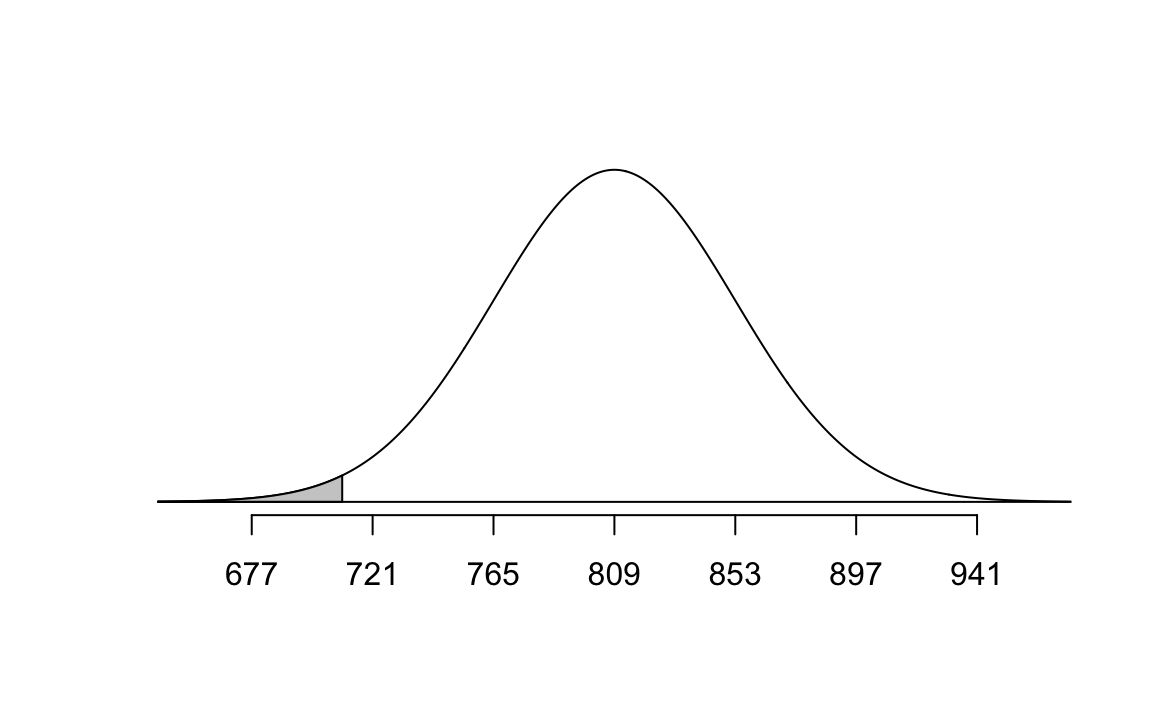
pnorm(q = mahogany, mean = bone_density_mean, sd = bone_density_se)[1] 0.01222447Exercise 10
Explain how your answers differ in similar sounding earlier vs. later exercises.
The probabilities are much smaller for the later exercises (sampling distribution) compared to the earlier (population distribution).
ggplot(
  data = tibble(x = c(bone_density_mean - bone_density_sd*3, bone_density_mean + bone_density_sd*3)),
  aes(x = x)) +
  stat_function(
    fun = dnorm,
    args = list(mean = bone_density_mean, sd = bone_density_sd)
  ) +
  stat_function(
    fun = dnorm,
    args = list(mean = bone_density_mean, sd = 44),
    linetype = "dashed",
    color = "blue"
  ) +
  geom_vline(
    xintercept = c(plywood, pine, mahogany),
    color = c("#deb887", "#01796f", "#c04000"),
    linewidth = 1
  ) +
  annotate(
    geom = "label",
    x = c(plywood, pine, mahogany),
    y = c(0.006, 0.007, 0.008),
    color = c("#deb887", "#01796f", "#c04000"),
    label = c("plywood", "pine", "mahogany")
  ) +
  annotate(
    geom = "text",
    x = 1000, y = 0.0018,
    label = "Population\ndistribution",
    hjust = 0,
    fontface = "bold"
  ) +
  annotate(
    geom = "text",
    x = 875, y = 0.005,
    label = "Sampling\ndistribution",
    hjust = 0,
    fontface = "bold",
    color = "blue"
  )